Exploring Mortgage Lending Data
Putting the Tools to Work on Real Data
With Jupyter, pandas, and matplotlib set up, let's put those tools to work on real data.

The Data
I'm using publicly available HMDA data, which stands for Home Mortgage Disclosure Act. Since 1975, most mortgage lenders in the US have been required to report detailed information about their lending activity. The Consumer Financial Protection Bureau publishes this data annually, and anyone can download it from ffiec.cfpb.gov/data-browser.
For community banks, HMDA data matters. Regulators use it to assess whether banks are serving their communities fairly. It feeds into CRA (Community Reinvestment Act) examinations. It reveals lending patterns across geography, loan types, and borrower demographics. Understanding how to work with this data is directly relevant to the regulatory environment banks operate in.
I downloaded 2021 data for Pennsylvania to keep the file size manageable. The full national dataset runs into tens of millions of records. Pennsylvania is a good pick because the Philadelphia metro area is one of the largest mortgage markets on the East Coast, and the state has enough geographic diversity to make the analysis interesting.
Loading and First Look
import pandas as pd
import matplotlib.pyplot as plt

df = pd.read_csv('hmda_2021_pa.csv')
print(f"Records: {len(df):,}")
df[['activity_year', 'loan_type', 'loan_purpose', 'loan_amount',
    'action_taken', 'state_code', 'county_code', 'income']].head()
Records: 863,993
   activity_year  loan_type  loan_purpose  loan_amount  action_taken state_code  county_code  income
0           2021          1            32        75000             1         PA        42101     159
1           2021          1            32       175000             1         PA        42133     131
2           2021          1            31       215000             4         PA        42077     150
3           2021          1             1       235000             4         PA        42101      45
4           2021          1            31        95000             4         PA        42133     130
Nearly 864,000 loan records from one state in one year. The columns use numeric codes rather than labels. Loan type 1 is conventional, 3 is VA. Loan purpose 1 is purchase, 31 is refinance. Action taken 1 means the loan was originated. The county_code field uses standard FIPS codes from the Census Bureau, so 42101 is Philadelphia County. The CFPB publishes a complete data dictionary with every field definition and valid code value, which is worth bookmarking if you plan to work with this data.
What Happened to These Applications?
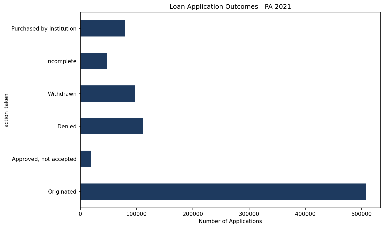
The action_taken field tells us the outcome of each application.
action_counts = df['action_taken'].value_counts().sort_index()
action_labels = {
    1: 'Originated',
    2: 'Approved, not accepted',
    3: 'Denied',
    4: 'Withdrawn',
    5: 'Incomplete',
    6: 'Purchased by institution'
}
action_counts.index = action_counts.index.map(lambda x: action_labels.get(x, f'Other ({x})'))
action_counts
Originated                  507,990
Approved, not accepted       18,948
Denied                      111,574
Withdrawn                    97,634
Incomplete                   47,643
Purchased by institution     79,262
About 59% of applications resulted in originated loans. Another 13% were denied. What caught my eye is that denials outnumbered withdrawals. I half expected the opposite during the 2021 refi boom, when people often shop several lenders at once and let the extra applications lapse. When the data doesn't match your hunch, that's usually where the interesting questions start.
action_counts.plot(kind='barh', figsize=(10, 6), color='#1e3a5f')
plt.title('Loan Application Outcomes - PA 2021')
plt.xlabel('Number of Applications')
plt.tight_layout()
Loan Types and Amounts
How do conventional loans compare to government-backed loans?
loan_type_labels = {1: 'Conventional', 2: 'FHA', 3: 'VA', 4: 'USDA'}
df['loan_type_name'] = df['loan_type'].map(loan_type_labels)

df.groupby('loan_type_name').agg({
    'loan_amount': ['count', 'mean', 'median']
}).round(0)
                 count      mean    median
loan_type_name
Conventional    711,919  225,032  175,000
FHA              96,556  187,207  165,000
USDA              7,163  162,225  155,000
VA               48,355  243,566  215,000
Conventional loans dominate at 82% of volume. VA loans average $243,566, close to conventional, reflecting the purchasing power of military borrowers. FHA and USDA serve lower price points at $165,000 and $155,000 median respectively, fulfilling their mission of expanding homeownership access. The relatively small USDA count makes sense for Pennsylvania, where eligible rural areas are limited compared to more agricultural states.
Denial Rates by Loan Type
This is where it starts to get interesting. Are denial rates consistent across loan types?
# Filter to just applications (not purchases)
applications = df[df['action_taken'].isin([1, 2, 3, 4, 5])]

# Calculate denial rate by loan type
denial_by_type = applications.groupby('loan_type_name').apply(
    lambda x: (x['action_taken'] == 3).sum() / len(x) * 100
).round(1)

denial_by_type.sort_values(ascending=False)
loan_type_name
FHA             14.5
Conventional    14.3
VA              13.2
USDA             7.9
dtype: float64
FHA has the highest denial rate at 14.5%, which fits, since these borrowers typically have lower credit scores and less saved for a down payment. What I didn't expect is how close conventional sits at 14.3%, just 0.2 points behind. I'd have guessed a wider gap between the two. USDA remains the lowest at 7.9%, likely because those loans go through pre-qualification before a formal application.
Raw denial rates only tell part of the story. The real question is whether those rates vary by borrower demographics, which is where fair lending analysis begins.
Geographic Patterns
Which counties have the most lending activity?
county_activity = df[df['action_taken'] == 1].groupby('county_code').size()
top_counties = county_activity.nlargest(10)
top_counties
county_code
42003    51,395
42101    47,274
42091    44,197
42017    34,071
42029    30,307
42045    24,255
42071    22,166
42133    22,015
42011    16,084
42077    14,880
dtype: int64
County 42003 is Allegheny (Pittsburgh) and 42101 is Philadelphia. Pittsburgh edges out Philadelphia in raw county-level originations. But the Philadelphia story changes when you look at the metro area. Four of the next five counties on the list are Philadelphia's collar counties. Montgomery (42091), Bucks (42017), Chester (42029), and Delaware (42045) together with Philadelphia account for over 180,000 originated loans, roughly 35% of all lending in the state. The Philadelphia metro area is by far the dominant mortgage market in Pennsylvania.
Income Distribution of Approved Loans
What does the income distribution look like for borrowers who actually got loans?
originated = df[df['action_taken'] == 1]
income = originated['income'].dropna()
income_clean = income[(income > 0) & (income <= 300)]

plt.figure(figsize=(10, 6))
income_clean.hist(bins=50, color='#0d9488', edgecolor='white')
plt.title('Income Distribution of Originated Loans - PA 2021')
plt.xlabel('Applicant Income ($000s)')
plt.ylabel('Number of Loans')
plt.axvline(income_clean.median(), color='red', linestyle='--',
            label=f"Median: ${income_clean.median():.0f}k")
plt.legend()
plt.tight_layout()
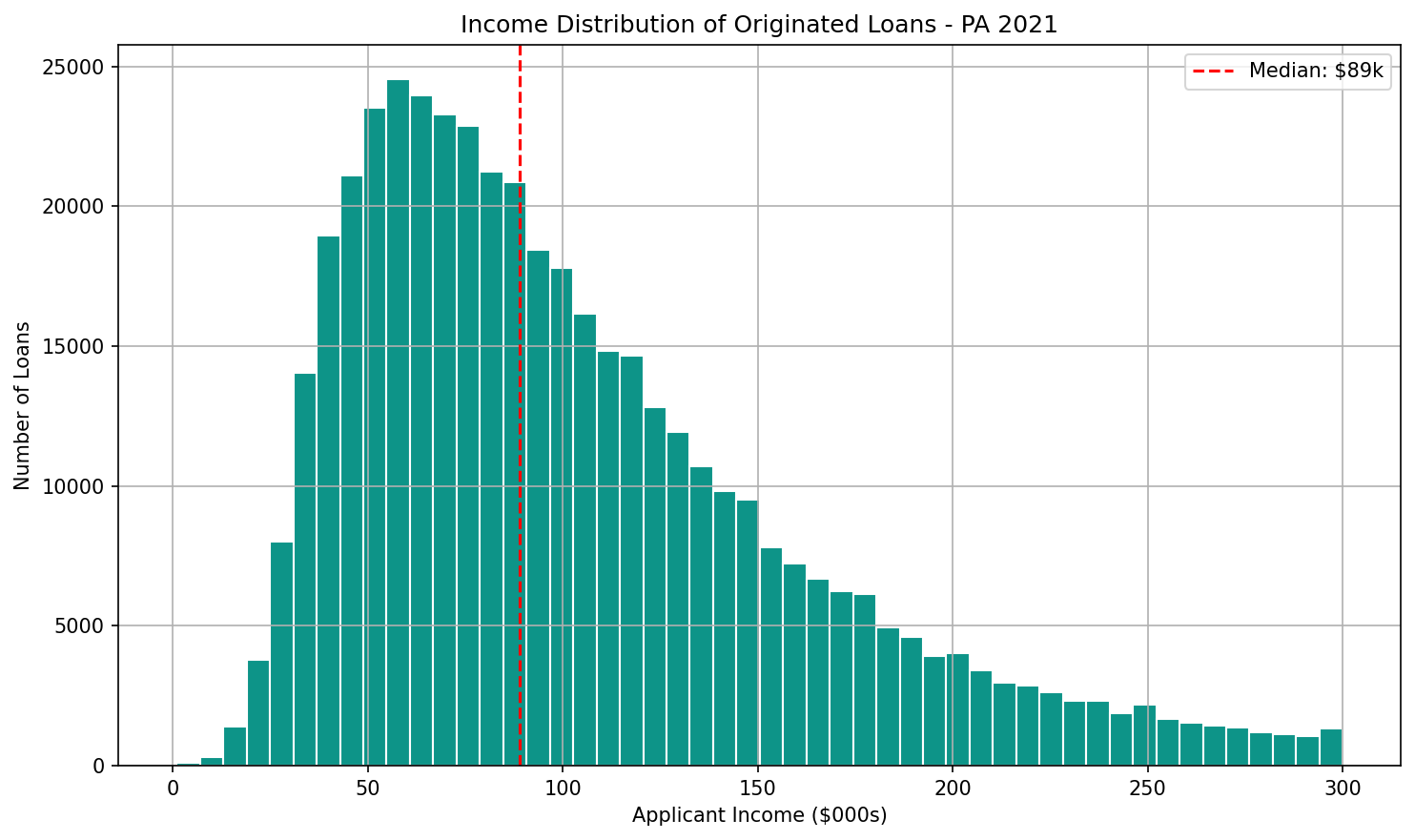
The distribution is right-skewed, with most borrowers earning between $40,000 and $150,000. The median is $89,000. There's a long tail of higher-income borrowers, which is typical for mortgage data and reflects the Philadelphia metro's mix of moderate-income neighborhoods and affluent suburban corridors.
What This Reveals
A single morning with HMDA data surfaces patterns that would take weeks to compile by hand. Denial rates cluster tightly across loan types in Pennsylvania. Lending concentrates heavily in the Philadelphia metro area. Income distributions shift based on how you slice the data.
This is what data exploration looks like in practice. You start with broad questions, run simple aggregations, and let the numbers guide you toward more specific inquiries. Some findings confirm what you'd expect. Others raise questions worth investigating further.
For a community bank, this kind of analysis connects to CRA planning, fair lending monitoring, and plain market understanding. And because HMDA data is public, anyone can benchmark an institution against the broader market using nothing but published records.